Re-Engineering Karnosky-Singer: Utility, Versatility and Insight for Practical Multi-currency Management

INTRODUCTION

In 1994, Denis S. Karnosky, Ph.D. and Brian D. Singer, CFA published a monograph entitled “Global Asset Management and Performance Attribution” (KS). They presented the idea that – due to the arbitrage known as interest rate parity – some contribution to the total return of a multi-currency portfolio is known, and ‘baked into’ a foreign-currency investment at the time it is made. Because this contribution is knowable and hedge-able, it should accrue to the currency market allocations of the manager – whether or not these are ultimately hedged.

While hugely influential among asset managers globally, these ideas remain largely unexploited in current performance practice. Though KS fully detail an attribution approach based on an expansion of the Brinson-Fachler method, and though this method is implemented in several commercially available performance systems – it is rarely adopted in the field.

We posit this circumstance to have arisen from several causes: misalignments between the paper’s formulation and practical investing reality, as well as inaccurate readings of, and consequently flawed implementations of the attribution method it sets out. We explore these causes in detail, and how they contribute to attribution results that fail to explain portfolio performance, obscuring the otherwise substantial value of KS’ central premise.

Finally, we develop a re-statement of KS that addresses those issues, producing an accurate decomposition of multi-currency effects that precisely explains the portfolio’s performance, while preserving the original paper’s essential insight. We go further to generalize this method and demonstrate its applicability to any investment attribution methodology.

INTEREST RATE PARITY AND KARNOSKY-SINGER

Interest rate parity derives from a true arbitrage that inextricably links foreign exchange (FX) spot and forward markets to international interest rates. The basic arbitrage is structured as follows:

• Borrow money in base currency for 1 period, at base cash rate
• Use this immediately to buy foreign currency F in the FX spot market
• Lend your currency F out for 1 period, at F’s local cash rate
• Sell currency F (plus interest received) for base currency, in the 1-period forward FX market.
• At the end of the period, unwind: collect F with interest, deliver on the forward contract and pay off the original loan in base, with interest.

Because this strategy requires no initial investment and is risk-free (excluding, say, counter-party risk), it must always realize a zero return.[1] Therefore, in an internationally invested portfolio, interest rate parity can be paraphrased in the following relationships[2]:

FX(forward) * (1 + Cash(foreign)) = FX(spot) * (1 + Cash(base))

FX(forward) / FX(spot) = (1 + Cash(base)) / (1 + Cash (foreign))

Where:

• FX(spot) is the spot price of one foreign currency unit, in base currency
• FX(forward) is the 1-period forward price of one foreign currency unit, in base currency
• Cash(base) is the 1-period interest rate in the base currency market
• Cash(foreign) is the 1-period interest rate in the foreign currency market

These equations make definitive statements about interest rate parity and its effect on foreign investing. The first equation says, “What you make/lose on the foreign side, you will lose/make on the base side.” The second equation puts it differently, “What you make/lose on the FX market, you will lose/make in the cash rate market.”

In the monograph now commonly known as Karnosky-Singer (KS), the authors make use of interest rate parity to point out that, at the beginning of an investment period, a portion of that period’s return is knowable and unavoidable. The size and direction of this contribution is based on the “difference”[3] between base and foreign cash rates. As they put it:

“Whether an investor decides to manage the currency exposure or not is irrelevant in developing the analytical framework; the portion of portfolio return that is attributable to currency must reflect a return that investors could actively manage.”

They go on to advocate that this effect be separate and measured independently in any multi-currency return attribution:

“This framework also allows the aggregate currency strategy to be evaluated independently of the stock, bond, and cash market decisions. This separation is critical not only for investment analysis but also for performance attribution.”

Together these statements declare that an international investment manager is responsible for more than just the naïve local market return; they are also responsible for return generated from their allocations to foreign currencies due to interest rate differentials from base currency. This responsibility is incurred whether the portfolio is hedged or not, whether the manager is responsible for implementing the hedge or not – in truth whether or not the manager has read the paper.

KS ATTRIBUTION:  A GAP BETWEEN INSIGHT AND PRACTICE

The immutable reality of interest rate parity (or ‘cash rate differential’) and its effect on international portfolios is now commonplace among professional global managers, traders and currency management desks, to be ignored only at one’s peril. Both strategic and tactical currency allocation decisions depend heavily on this critical factor.

Why, then, when it comes to performance attribution, do we so rarely find the KS methodology being utilized? Most commercially available performance systems offer it as an option, but to paraphrase what we’ve heard from several vendors, “Few (or none) of our clients have implemented Karnosky-Singer attribution.”

We posit two over-arching causes for this apparent shortfall:  formulation of the methodology, and its implementation.

SHORTCOMINGS OF FORMULATION:  THEORY AND PRECISION

The original formulation of the insights of KS exhibit, from the start, several obstacles to a manger seeking an accurate and consistent representation of their currency allocation and hedging performance.

First, the formulas presented by KS in their framework are based entirely in continuously compounded return space; whereas in practice, a manager’s input data and performance results are expressed solely as periodic returns. While returns can be converted one to the other straightforwardly, the outputs of attribution – i.e., contributions to portfolio return and management value-added – are not so tractable.

Second is the matter of precision and ‘residuals.’  As KS observe in their footnote 12, there is a seventh effect (cross-product) which they state to be “a relatively small term.” However, as managers well know, an effect which is small 99% of the time is likely to generate a big – and, if missing, unexplainable – impact, twice a year.

Finally, KS provides valuable insights into the generators of portfolio performance – absolutely, even without benchmark relative effects. KS is not, at its core, an attribution methodology, but instead a decomposition of currency allocation contributions to portfolio return. As such, it can be successfully applied to benchmarks, and in the context of any attribution methodology whatsoever. In general practice; however, this method is applied almost exclusively to the Brinson-Fachler method – resulting in a coupling that is now commonly referred to as “Karnosky-Singer attribution.” This misinterpretation has pushed away many managers whose investment processes, and consequent attribution requirements, do not align with an Allocation/Selection framework.

SHORTCOMINGS OF IMPLEMENTATION

To further worsen matters, these flaws in KS’ formulation have been replicated and magnified in many implementations. Some have blindly copied the continuous-compounding formulas into code, and then fed periodic rates to these as inputs. Needless to say, the attributions that result generate substantial and (usually) unacceptable variances from realized performance.

The formal construction of KS attribution in the paper consisted of six separately measured effects. In their examples; however, they combined these variously to report on only three. Consequently, most attribution implementations also support only these three effects, denying managers granularity and the ability to combine along different axes, telling a story aligned with their proprietary investment process.

Another assumption of KS which does not compare well with investment reality is that of a perfect, single-period hedge. Hedging, in practice, is generally not implemented for single, regular periods – particularly when the analytic periodicity is daily. Even in a monthly context, different currencies may be more efficiently hedged with different frequencies, calendars and roll dates. Furthermore, it is often the case that currencies with relatively illiquid forward markets are hedged with more liquid proxies that correlate only approximately.

We have found that any one of these shortcomings – let alone the aggregate weight of them all – is usually enough to cause a manager to look beyond available ‘Karnosky-Singer attribution’ options for their attribution solution.

RETURNING INSIGHT TO MODERN MULTI-CURRENCY MANAGEMENT

This article is not the first to observe or confront these impediments in a modern investment context. In their article, Menchero and Davis (2009) directly address several of the shortcomings listed above, including formulation in periodic return space, restoration of the cross-product and application to other attribution methodologies (including factor-based attribution), to great success.

We have taken a somewhat different approach, with similar ends. To be specific, we intend to look at the methodology more from the point of view of an engineer looking to build or ‘re-engineer’ a KS framework, and less from a theoretical perspective. In the context of that objective, we have adopted some methodological guidelines:

• Make the inputs and outputs informative to actual investment processes and practices. Most importantly, we recast the KS methodology to both consume and produce periodic data.
• Use only readily available input data. Here we have made use of cash rate curves and FX spot and forward curves, rather than currency returns.
• Ensure accuracy, eliminate residual. To that end, we restore the cross-product effect, reflecting the interaction of market and currency management decisions.
• Accommodate real-world hedging. Attribution effects from hedging are separated, and performance measured using market inputs and valuations. Furthermore, we explicitly measure performance of forwards that have been initiated before the beginning of, and/or have deliveries beyond the end of the performance period, and forwards that are proxy hedges for other currencies.
• Preserve attribution granularity in calculation; aggregate in presentation. We restore the attribution to its full, granular decomposition, and show examples of how these might be aggregated to illustrate different attribution stories.
• Apply to multiple attribution methodologies. We de-couple the KS decomposition from its original Brinson-Fachler attribution; thereby showing that the central thesis of KS can be valuably applied to any methodology, including strategy-, process- and decision-based attributions.

Finally, we think all these objectives and guidelines are more clearly (and often, more accurately) addressed as calculations of gain/loss and contribution to portfolio return.[4] In the presence of intra-period transactions and transaction-based returns, questions and decisions around flow-weighting can often confuse the meaning and intent of calculations specified in terms of weight and return. All of the formulas presented[5] can be readily adapted, should one wish, to weight and return space, given the choice of an appropriate Denominator.[6]

KS ATTRIBUTION EFFECTS:  A DECOMPOSITION

Now we begin to specify the “effects” of KS – specifically, the decomposition of performance at every level (position, bucket, portfolio) into its root causes, according to the methodology. First, we begin with what we’ll call the ‘naïve’ effects, calculated without recognition of the known performance generated by interest rate parity. All effects will be expressed in terms of gain/loss, in base currency of the portfolio.

Asset Level Effects

First we calculate effects generating gain/loss for the primary assets of the portfolio, exclusive of the hedging positions.

• Naïve local market – This effect represents the total gain/loss generated by rise/fall of the asset’s value in its local market. Simply take the gain/loss of the asset in foreign currency and convert to base currency at the beginning-of-period (BoP) exchange rate.
• Naïve FX – Naïve FX is the total gain/loss generated by the observed change in spot exchange rates. Convert BoP exposure in local currency to base currency, at both BoP and end-of-period (EoP) exchange rates. Then subtract to arrive at change over the period.
• Cross product – Cross Product measures the interaction between the local market and exchange rate fluctuations. Whereas the prior effects measure performance of the BoD exposure only, Cross Product measures the gain/loss due to the FX market on the gain/loss generated by the local market. It is less intuitively calculated as Naïve Local Market times Naïve FX, as a percentage of the BoD exposure of the asset.

These three effects, thus far, constitute a complete decomposition of the asset’s performance: i.e., their sum will equal the total gain/loss of the asset in base currency. However, they are as indicated by their names, naïve – they fail to take into account the known interest rate differential between foreign and base currencies, and thus include its performance incorrectly in the Naïve local market effect. First, we must calculate the Interest rate effect, then transfer it to its proper KS location.

• Local rate – This effect is simply the gain/loss on the asset given its local periodic cash interest rate, expressed in base currency. Multiply the BoD base currency exposure by the BoD periodic local market cash rate.
• KS local market – The Interest rate performance is incorrectly included in the Naïve local market effect, so we simply subtract it from there to arrive at KS local market premium…
• KS FX – … and add it back into the Naïve FX effect, where it belongs, to end up with KS FX.

The KS decomposition of the asset’s total gain/loss is now KS local market + KS FX + Cross product.

Hedging Effects

Because we wish to measure the performance provided by actual hedge instruments employed in the portfolio, as opposed to theoretical ‘perfect’ hedges, we decompose the total hedge gain/loss[7] separately and differently, based on the observed gain/loss of these positions.

• Total hedge – Total hedge effect is simply the gain/loss, over the attribution period, of the actual hedging instrument.
• Native hedge – Native hedge is one where the foreign currency is the same as the assets it is being used to hedge, and the currency being hedged to is base. For hedging instruments that are native, Native hedge equals Total hedge. For non-native or ‘proxy’ hedges, Native hedge is the gain/loss of a hypothetical native hedging instrument, held in the same base notional amount and delivery as the actual (proxy[8]) hedge.
• Proxy hedge – Proxy hedge is the difference between Total hedge and Native hedge, i.e., the gain/loss derived from using a proxy hedge rather than a native one. Therefore, for all native hedges, the Proxy hedge effect will be zero.
• Roll – Hedging can be further decomposed into Roll and FX change effects. Roll represents the gain/loss derived from the fact that the time to delivery, over the course of the period, becomes one period shorter and thus ‘rolls’ down the FX forward curve generating gain/loss. Calculate as the difference in value between: a) a hypothetical hedge instrument, identical but one period shorter to delivery, and b) the actual hedge instrument’s BoD market value.
• FX Change – This effect is simply the remainder of the hedge’s effect after Roll due to FX market fluctuation. For Native hedges, FX change is Native hedge minus Roll. For proxy hedge it is the difference between the actual and native FX Change effects.

PRESENTATION OF EFFECTS:  TELLING THE INVESTMENT STORY

At this point, we’ve decomposed portfolio performance to its most granular sources, based on the KS methodology augmented by a more real-world approach to hedging. Why did we go to such lengths to measure so many separate effects with such detail?

Although it is possible to present a report that breaks out each KS effect separately, such a report would likely be unwieldy and confusing. Generally, we’ll find it more comprehensible to combine effects into a more compact set, one specifically tailored to measure the components of the manager’s proprietary investment process and their performance. The advantage of calculating at a granular level and then combining for presentation is that we are thus able to combine flexibly along axes that best suit the report’s purpose. Let’s have a look at some examples.

For a global asset manager, allocation decisions along axes other than currency are equally important. The KS inclusion of interest rate differential effects in the manager’s local market performance guarantees an accurate view of local market vs. FX performance for each asset class, or indeed for any allocation segment.

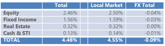
Here the manager can see the breakout of total performance by sector, broken into local and FX components. The decomposition is:

• Local Market = KS local market
• FX Total = KS FX + Cross product + Total Hedge

Another manager, allocating by currency exposure, might need to delve deeper into the root sources of currency gain/loss, as hedged:

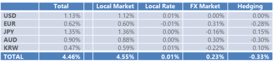
• Local Market = KS local market
• Local Rate = Local rate
• FX Market = Naive FX + Cross product
• Hedging = Total hedge

As a final example, a manager responsible for hedge implementation would want to focus with greater precision on hedge-specific performance effects:

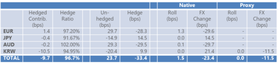
• Not included = KS local market and Cross product
• Hedge % = – Hedge exposure/total foreign currency exposure
• Un-hedged = KS FX
• Hedge = Total Hedge
• Last 4 columns = as named

FROM DECOMPOSITION TO ATTRIBUTION

To this point, the analysis has been simply a decomposition of portfolio performance. Our final objective is the application of this method directly to one or more benchmarks comparatively, i.e., attribution.

As did KS, we can apply the decomposition to arrive at Allocation and Selection effects:

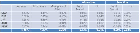
• Management Effect = Portfolio total performance – Benchmark total performance
• Allocation Local Market = KS local market of the Allocation notional portfolio
• Allocation FX = KS FX + Cross product of the Allocation notional portfolio
• Selection Local Market = KS local market of the Selection + Interaction notional portfolio
• Selection FX = KS FX + Cross product of the Selection + Interaction notional portfolio

However, the KS method is not intrinsically coupled with Brinson-style attribution. Because it is, instead, a simple decomposition of performance within a portfolio, it can be applied to any comparison of actual and benchmark (or other notional) portfolios. Thus, its versatility is extensible to the measurement of any proprietary investment process. To illustrate, a typical process-based attribution:

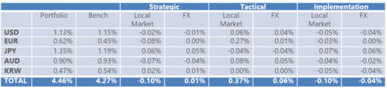
• Local Market = the differences in KS local market from the benchmark to Strategic, to Tactical to actual portfolios progressively
• FX = the differences in KS FX + Cross product from the benchmark, to Strategic, to Tactical to actual portfolios progressively

Many other methodologies affording insight into proprietary investment processes – e.g., strategy- and decision-based attribution – can be similarly extended with the KS formulations; such versatility makes it a very powerful tool for the performance practitioner.

FURTHER OPPORTUNITIES:  OTHER APPLICATIONS, INCREASED PRECISION

The methodology we’ve presented thus far is exact and fit-for-purpose as it stands. Nevertheless, the domain of multi-currency management comprises many objectives, employing a wide variety of strategies; broader applications and greater precision will often be required[9]. We suggest here some opportunities for further development.

Multiple reviewers[10] have pointed out that we have focused exclusively on the manager hedging away foreign currency risk to a native base currency. While hedging is a common objective of a currency overlay, many other strategies require active currency management. KS point this out particularly well, particularly with regard to managing currency allocations in the presence of advantageous cash rate differentials. For the sake of brevity, we have limited current scope to hedging; generalization to currency overlays with other objectives is a worthy candidate for development.

While gain/loss incorporates performance from both BoD exposures and transactions, one may wish to measure their effects separately (particularly if transaction costs are of interest). In this case, it is important to capture the transacted prices and exchange rates of foreign currency assets and use this as the basis for calculating gain/loss for over the period (rather than BoD or EoD spot rates).

FX forward valuation is theoretically not very complex; but, because it is an inherently global exercise, the real-world intricacies introduced by multiple quote methods, sources and timings can produce measurable attribution effects as well as unwanted artifacts. The differences among the valuation methodologies of the accounting system, the benchmark and the market can all be measured, decomposed and attributed, if the underlying assumptions and data points can be assembled[11]. Further dissection of differences between benchmark and portfolio hedge rolling policy presents another avenue of investigation.

Finally, we’ve used in our calculations a single-point quote for FX and cash rates. In reality, these exist and are obtainable as bid-ask spreads. For a finer degree of precision, the appropriate side of the trade can be selected and used in the attribution calculation. This is often particularly desirable for managers who maintain both long and short asset exposures to foreign currencies.

CONCLUSION

For decades, the Karnosky-Singer monograph of 1994 has provided crucial insight into the performance of foreign asset allocation and hedging. While this information has been effectively absorbed into management process and portfolio construction, its use in ex-post attribution has lagged. We believe this to be due to structural issues with the original formulation, combined with misinterpretation of its findings during implementation.

We have presented a re-formulation of the key concepts introduced by KS, with the intention of promoting its implementation and use by making it simple, flexible, extensible and feasible to implement, given real-world data sources and investment practices.

HOW MERADIA CAN HELP

Meradia, with its staff of industry-recognized experts and influencers, has a long history of innovation and quality delivery in the investment performance and front-office domains. We specialize in identifying and assembling the bespoke set of method, technique, data and technology that best supports the client’s proprietary investment practice.

APPENDIX – ATTRIBUTION FORMULAS

This appendix details the formulaic calculations required for use in the re-engineered Karnosky-Singer performance framework.

Inputs – Single-period inputs to the calculations

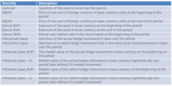
Outputs

Naïve Local Market = GL(local) * X(BoP)

Naïve FX = E(local, BoP ) * [ X(EoP) – X(BoP) ]

Cross Product = Naïve Local Market * Naïve FX / [ E(local, BoP) * X(BoP) ]

Interest Rate = E(base, BoP) * C(local, BoP)

KS FX = Naïve FX – Interest Rate

KS Local Market = Naïve Local Market + Interest Rate

Total Hedge = HGL(actual, base)

Native Hedge = HGL(native, base)

Proxy Hedge = HGL(actual, base) – HGL(native, base)

Native Roll = HV(native, base, +1) – HV(native, base, BoP)

Native FX Change = Native Hedge – Native Roll

Proxy Roll = HV(actual, base, +1) – HV(actual, base, BoP)  – Native Roll

Proxy FX Change = Proxy Hedge – Proxy Roll

All above outputs are expressed as gain/loss amounts. To convert any of the (GL) quantities to a contribution-to-portfolio-return (CTR):

CTR = GL / Market value of the portfolio at BoP

Aggregation of asset-level GL and CTR quantities up to bucket and portfolio levels is completely additive.

Should one wish to further transform these effects into returns (R) and weights, an appropriate flow-weighting method for transactions must be selected and a consistent Denominator (D) be calculated at the asset level:

R = GL / D

W = D / Market value of the portfolio at BoP

DOWNLOAD A SPREADSHEET TO INVESTIGATE & CONFIRM COMPUTATIONAL FORMULAE

REFERENCES

Karnosky, Denis, and Brian D. Singer, “Global Asset Management and Performance Attribution,” The Research Foundation of the Institute of Chartered Financial Analysts, Volume 1994, Issue 3

Menchero, Jose, CFA and Davis, Ben, Ph.D., “Multi-Currency Performance Attribution” The Journal of Performance Measurement, Fall 2009, Vol. 6 No. 3, pp. 47-55

END NOTES

[1] In reality, the arbitrage return is almost always slightly negative. Even when attempting to reverse the direction of the arbitrage, bid-ask spreads generate a small loss.

[2] These are the only formulas we will present in the body of the article. The Appendix contains a full formulaic expression of the methodology described therein.

[3] In KS’ formulation, using continuously compounded rates of return, the arithmetic difference between base and foreign cash rates. In periodic return space, as we see, it is instead a ratio of 1 + rates.

[4] We have observed several firms, in recent experience, arrive at this same conclusion; “Dollar-based” attribution is becoming more popular.

[5] See the appendix.

[6] Much has been written on transaction flow-weighting methods, and the appropriate choice of denominator. By expressing the methodology in terms of gain/loss and contribution, we hope to remove these considerations from the scope of this article, as well as extend its applicability to any choice of flow-weighting method.

[7] Valuation of FX forwards, while not especially difficult, is complicated by quote conventions used in trading, which can be currency-specific regarding direction and scaling. Essentially, the value of an FX forward is the cumulative gain/loss on the position since it was opened (at which time, it is zero). To maintain focus on the main topic of this article, we assume this value has been supplied, prior to attribution, by another source such as an accounting system or other valuation engine.

[8] Proxy hedges are commonly employed when the FX forward market for the foreign currency is relatively illiquid or otherwise expensive to trade.

[9] Index fund attribution, for example.

[10] Many thanks to Russ Glisker and Jose Michaelraj.

[11] Which can present challenges, particularly in the case of the benchmark, and possibly more so when accounting valuations are outsourced.

Download Thought Leadership ArticleServices: Solution DesignExpertises: Performance, Risk & AnalyticsClients: Asset ManagersAuthors: Meradia Consultant